How Uniswap works
Contents
[1]:
# we use bokeh for plotting
from bokeh.io import output_notebook, show
from bokeh.layouts import column
from decimal import Decimal

output_notebook()
How Uniswap works#
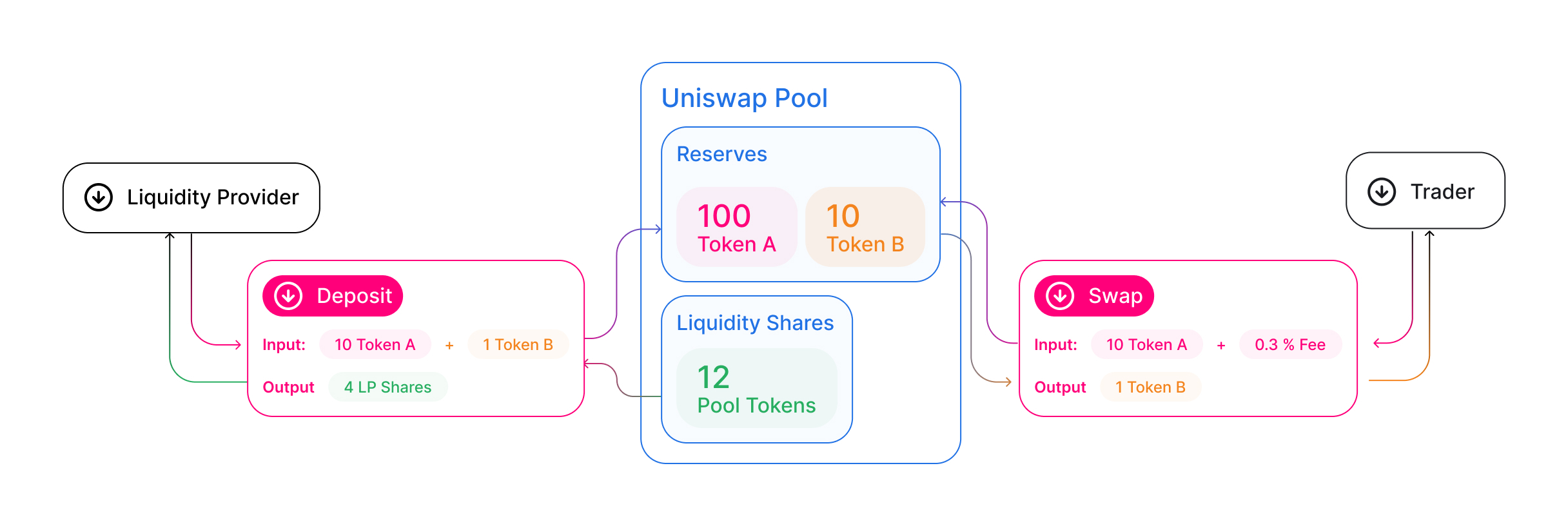
Uniswap is an automated liquidity protocol powered by a constant product formula and implemented in a system of non-upgradeable smart contracts on the Ethereum blockchain. It obviates the need for trusted intermediaries, prioritizing decentralization, censorship resistance, and security. Uniswap is open-source software licensed under the GPL.
Each Uniswap smart contract, or pair, manages a liquidity pool made up of reserves of two ERC-20 tokens.
Anyone can become a liquidity provider (LP) for a pool by depositing an equivalent value of each underlying token in return for pool tokens. These tokens track pro-rata LP shares of the total reserves, and can be redeemed for the underlying assets at any time.
[2]:
from cpy_amm.market import MarketPair, Pool, TradeOrder
from cpy_amm.swap import constant_product_swap
from cpy_amm.plotting import new_pool_figure

# liquidity pool made up of reserves of Token A
pool_token_A = Pool("A", 100)
# liquidity pool made up of reserves of Token B
pool_token_B = Pool("B", 100)
# create a market for A/B
mkt = MarketPair(pool_token_B, pool_token_A, 0.003, 0)
# amount of tokens A to swap in
trade_order = TradeOrder("A/B", 10, mkt.swap_fee)
# swap 10 tokens A for tokens B
constant_product_swap(mkt, trade_order)
# plotting the reserves before and after swap
p = new_pool_figure(pool_token_A, pool_token_B, steps=["Before Swap", "After Swap"])
# display plot
show(column(p, sizing_mode="stretch_both"))
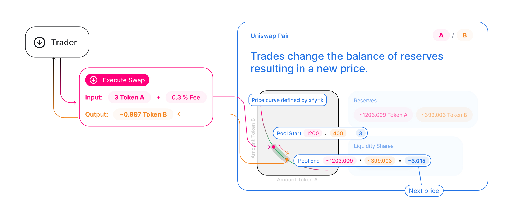
Pairs act as automated market makers, standing ready to accept one token for the other as long as the “constant product” formula is preserved. This formula, most simply expressed as x * y = k, states that trades must not change the product (k) of a pair’s reserve balances (x and y). Because k remains unchanged from the reference frame of a trade, it is often referred to as the invariant. This formula has the desirable property that larger trades (relative to reserves) execute
at exponentially worse rates than smaller ones.
Because the relative price of the two pair assets can only be changed through trading, divergences between the Uniswap price and external prices create arbitrage opportunities. This mechanism ensures that Uniswap prices always trend toward the market-clearing price.
⚠️ Please not that contrary to UNISWAP, we use the convention BASE/QUOTE. In our case Uniswap pair A/B corresponds to B/A eg. to buy the pair represented by the market you need to input the quote token, in this case A, to receive the base token, in this case B. The price however remains the same eg. A / B (Quote / Base)
[3]:
from cpy_amm.plotting import new_price_impact_figure

# liquidity pool made up of reserves of Token A
pool_token_A = Pool("A", 1200)
# liquidity pool made up of reserves of Token B
pool_token_B = Pool("B", 400)
# create a market for B/A with 0.03% fee
mkt = MarketPair(pool_token_A, pool_token_B, 0.003, 0)
# swap 10 A for B
trade_order = TradeOrder("B/A", 10, mkt.swap_fee)
# new plot with price impact of swapping 3 tokens A
p = new_price_impact_figure(mkt, trade_order)
# display plot
show(column(p, sizing_mode="stretch_both"))
First liquidity provider#
Each Uniswap liquidity pool is a trading venue for a pair of ERC20 tokens. When a pool contract is created, its balances of each token are 0; in order for the pool to begin facilitating trades, someone must seed it with an initial deposit of each token.
The first liquidity provider is the one who sets the initial price of the pool. They are incentivized to deposit an equal value of both tokens into the pool. To see why, consider the case where the first liquidity provider deposits tokens at a ratio different from the current market rate. This immediately creates a profitable arbitrage opportunity, which is likely to be taken by an external party.
[4]:
from cpy_amm.market import new_market, MarketQuote
from cpy_amm.swap import constant_product_swap
from cpy_amm.plotting import new_constant_product_figure, new_pool_figure

# USDT/USD market price
usdt_usd = MarketQuote("USDT/USD", 1)
# UNI/USD market price
uni_usd = MarketQuote("UNI/USD", 6.32)
# create a 10000 USD market for UNI/USDT with 0.3%
mkt = new_market(10000, usdt_usd, uni_usd, 0.003)
# new plot with constant product curve
cp_plot = new_constant_product_figure(mkt)
# swap 3000 USDT for UNI
trade_order = TradeOrder("UNI/USDT", 3000, mkt.swap_fee)
# swap
constant_product_swap(mkt, trade_order)
# plotting the reserves before and after the swap
pools_plot = new_pool_figure(mkt.pool_1, mkt.pool_2, steps=["Before Swap", "After Swap"])
# display plots
show(column(cp_plot, pools_plot, sizing_mode="stretch_both"))
Providing Liquidity#
When providing liquidity from a smart contract, the most important thing to keep in mind is that tokens deposited into a pool at any rate other than the current reserve ratio are vulnerable to being arbitraged. As an example, if the ratio of x:y in a pair is 10:2 (i.e. the price is 5), and someone naively adds liquidity at 5:2 (a price of 2.5), the contract will simply accept all tokens (changing the price to 3.75 and opening up the market to arbitrage), but only issue pool tokens entitling the sender to the amount of assets sent at the proper ratio, in this case 5:1. To avoid donating to arbitrageurs, it is imperative to add liquidity at the current price. Luckily, it’s easy to ensure that this condition is met!
[5]:
from cpy_amm.market import new_market, MarketQuote
from cpy_amm.swap import constant_product_swap
from cpy_amm.plotting import new_constant_product_figure, new_pool_figure

# USDT/USD market price
usdt_usd = MarketQuote("USDT/USD", 1)
# UNI/USD market price
uni_usd = MarketQuote("UNI/USD", 6.32)
# create a 10000 USD market for UNI/USDT
mkt = new_market(10000, usdt_usd, uni_usd, 0.003)
# new plot with constant product curve
cp_plot = new_constant_product_figure(mkt)
# USDT/USD new market price
usdt_usd = MarketQuote("USDT/USD", 1)
# UNI/USD new market price
uni_usd = MarketQuote("UNI/USD", 6.46)
# deposit 5000$ 3 times, mid price must not change
for _ in range(0,3):
    # add 5000$ liquidity using new market quotes
    mkt.add_liquidity(5000, usdt_usd, uni_usd)
    # new plot with constant product curve
    cp_plot = new_constant_product_figure(mkt, bokeh_figure=cp_plot)
# plotting the reserves before and after swap
pool_plot = new_pool_figure(mkt.pool_1, mkt.pool_2, steps=["L0", "L1", "L2", "L3"])
# display plots
show(column(cp_plot, pool_plot, sizing_mode="stretch_both"))
Constant Product AMM Order Book#
From the paper On Equivalence of Automated Market Maker and Limit Order Book Systems the equation for the cumulative quantity at any mid price is given by:
[6]:
from cpy_amm.market import new_market, MarketQuote
from cpy_amm.plotting import new_order_book_figure

# USDT/USD market price
usdt_usd = MarketQuote("USDT/USD", 1)
# UNI/USD market price
uni_usd = MarketQuote("UNI/USD", 6.32)
# create a 10000 USD market for UNI/USDT
mkt = new_market(10000, usdt_usd, uni_usd, 0.003)
# new plot with constant product curve
order_book_plot = new_order_book_figure(mkt, x_min=2000, x_max=8000)
# display plots
show(column(order_book_plot, sizing_mode="stretch_both"))
Autoviz for constant product AMMs#
[7]:
from cpy_amm.market import MarketQuote, MarketPair, new_market
from cpy_amm.plotting import cp_amm_autoviz

# initial liquidity in USD
deposit_usd = 10000
# USDT/USD market price
usdt_usd = MarketQuote("USDT/USD", 1)
# UNI/USD market price
uni_usd = MarketQuote("UNI/USD", 6.32)
# create a 10000 USD market for UNI/USDT
mkt = new_market(10000, usdt_usd, uni_usd, 0.003)
# display data
cp_amm_autoviz(mkt)